| votechoice | Favor | Neutral | Oppose |
|---|---|---|---|
| Biden | 0.503 | 0.041 | 0.027 |
| Trump | 0.162 | 0.133 | 0.134 |
POSC 8410: Joint Distributions
Describing two variables at once, covariance, and correlation
Will Horne
Where We Are
Everything so far has been about one random variable at a time
But most interesting questions in social science involve two or more
- Does income predict turnout? Does a name predict a callback?
Today: how two random variables behave together + baby steps towards regression
Joint Distributions
Two Variables at Once
The joint PMF of discrete \(X\) and \(Y\) gives the probability of every combination:
\[p_{X,Y}(x, y) = P(X = x, \; Y = y)\]
It must be non-negative
And it must sum to 1 over all pairs: \(\sum_x \sum_y p_{X,Y}(x,y) = 1\)
Same two rules as always. There are just two indices now.
You Have Already Seen This!
Vote choice and support for raising taxes on the rich, as proportions of the whole sample:
That is a joint PMF. The six cells sum to 1, and each is \(P(\text{vote} = v, \; \text{policy} = t)\).
Informally, we call these cross-tabs. Formally, they are joint distributions.
The Margins
To get the distribution of one variable alone, sum over the other:
\[p_X(x) = \sum_y p_{X,Y}(x, y)\]
| votechoice | P(vote choice) |
|---|---|
| Biden | 0.571 |
| Trump | 0.429 |
Called marginal distributions for a silly reason: they are the row and column totals, traditionally written in the margins of the table.
Conditional Distributions
Fix one variable, and renormalize:
\[p_{Y \mid X}(y \mid x) = \frac{p_{X,Y}(x,y)}{p_X(x)}\]
| votechoice | Favor | Neutral | Oppose |
|---|---|---|---|
| Biden | 0.882 | 0.071 | 0.047 |
| Trump | 0.377 | 0.309 | 0.313 |
Each row now sums to 1. Just conditional probability applied to a whole distribution.
Independence, Formally
\(X\) and \(Y\) are independent if the joint is the product of the marginals, for every pair:
\[p_{X,Y}(x,y) = p_X(x)\,p_Y(y)\]
Check one cell. \(P(\text{Biden}) = 0.571\) and \(P(\text{Favor}) = 0.665\):
The observed joint probability is 0.503. Not even close!
So, vote choice and tax policy views are strongly dependent.
Covariance
Do They Move Together?
Marginals tell us about each variable alone
Conditionals tell us about one given the other
Now we want a single number summarizing whether they move together
\[\text{Cov}(X,Y) = E\big[(X - E[X])(Y - E[Y])\big]\]
Help me out (I’ve forgotten all my stats knowledge!). Why is this a good measure - what is it doing?
Reading the Quadrants
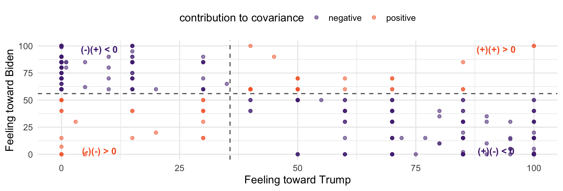
The dashed lines are the two means.
The Sign
Points above both means or below both means contribute positively
Points high on one and low on the other contribute negatively
Covariance is the average of those contributions
Here almost everything lands in the two negative quadrants: warm toward Trump goes with cold toward Biden. Negative covariance.
Covariance in Our Data
Negative, as the picture promised
But what does \(-1170\) mean?
The units are thermometer-points times thermometer-points. There is no such thing.
The Units Problem
Covariance depends entirely on the scale of your variables
Measure income in dollars instead of thousands and the covariance grows by a factor of 1,000
Note: \(\text{Cov}(aX, bY) = ab\,\text{Cov}(X,Y)\)
So the sign is meaningful and the magnitude is not comparable across variables. We need to standardize.
Correlation
Standardizing Covariance
Divide by both standard deviations:
\[\rho_{X,Y} = \frac{\text{Cov}(X,Y)}{SD(X)\, SD(Y)}\]
[1] -0.8159562[1] -0.8159562−0.82. Now it means something: warmth toward one candidate strongly predicts coldness toward the other.
Properties
Always between −1 and 1
\(\rho = \pm 1\) only if the points fall exactly on a straight line
Unitless — unaffected by rescaling either variable
Symmetric: \(\rho_{X,Y} = \rho_{Y,X}\)
If \(X\) and \(Y\) are independent then \(\rho = 0\). But the reverse does not hold — zero correlation does not imply independence. (why?)
Anscombe’s Quartet
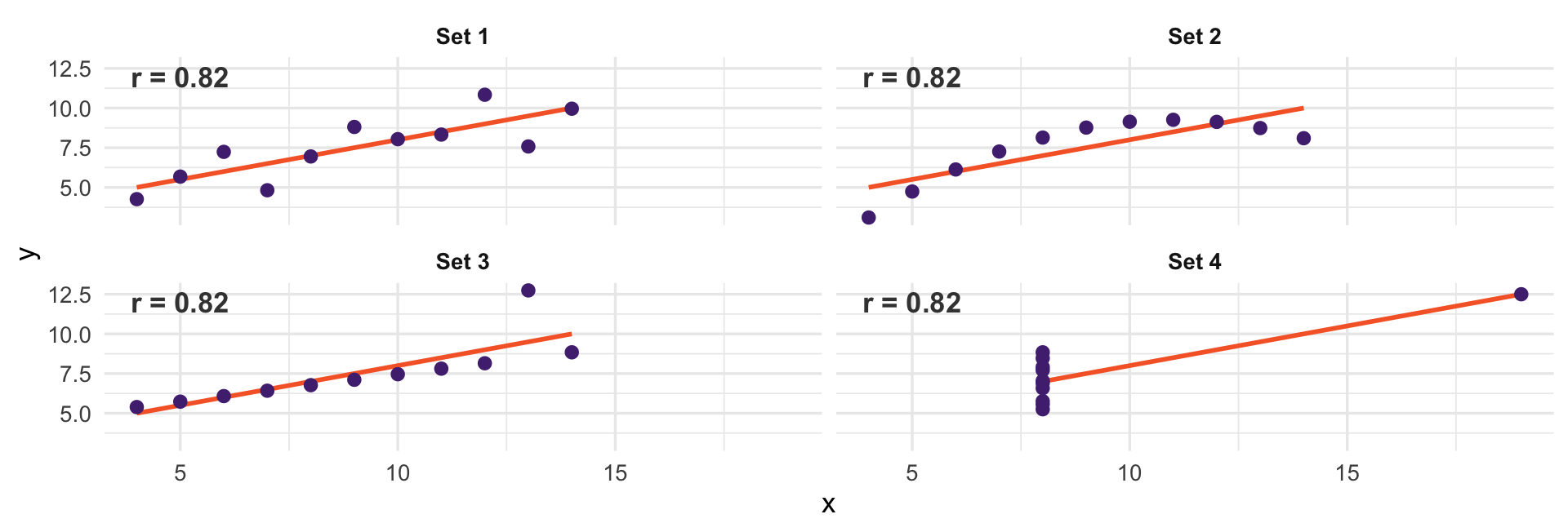
Four datasets. Identical correlations, identical regression lines. One is linear, one is curved, two are driven by a single point.
What Correlation Misses
It only sees linear association. Set 2 is a perfect curve and still reports 0.82
It is not robust. Sets 3 and 4 are decided by one observation
The Bridge to Regression
The Slope Is a Ratio
Soon we will fit \(Y = \beta_0 + \beta_1 X\) by least squares. The answer will turn out to be:
\[\beta_1 = \frac{\text{Cov}(X, Y)}{\text{Var}(X)}\]
The numerator: how \(X\) and \(Y\) move together
The denominator: how much \(X\) moves at all
A regression slope is co-movement per unit of variation in the predictor
Check It
[1] -0.7288199 ft_trump
-0.7288199 Identical. We have already computed a regression coefficient
You Try
Build the joint distribution of
votechoiceandacaas proportions of the whole sample. Do the cells sum to 1?Get the marginal distribution of
acafrom it.Compute the conditional distribution of
acagivenvotechoice. Which rows sum to 1?Compute
cor(ft_science, ft_fauci). Then compute the regression slope by hand usingcovandvar, and check it againstlm.
For Next Time
Read: Blitzstein and Hwang, Sections 7.1–7.5
Next class: conditional expectation — the mean of \(Y\) within levels of \(X\)
We computed one by hand in Week 2 with
group_by()It is the single most important object between here and regression