POSC 8410: Continuous Random Variables

The uniform, the normal, and probability as area

Will Horne

Where We Are

Last time: derivatives are marginal effects, and integrals are areas
Today we apply this to probability

Continous distributions replace summation with calculus

Continuous Random Variables

The Problem

Suppose $P(X = x) = \epsilon > 0$ for every $x$ in $(0,1)$.

How many real numbers lie between 0 and 1?

Uncountably infinite
So the total probability would be $\infty$
Violating the axiom that probability cannot exceed 1

So $P(X = x) = 0$

Let $X$ be uniform on $[0, 10]$.

$P(X = 3)$? Zero.
$P(X = 0.194345111223)$? Also zero.

This does not mean 3 cannot happen. It is in the support. For continuous variables, probability zero is not impossibility.

But it does mean the PMF is not helpful here! We need a different function.

Income

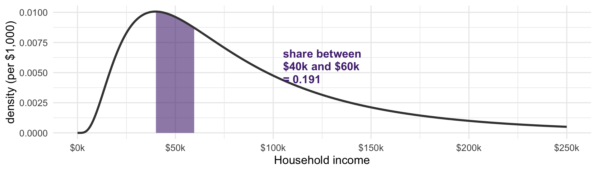
Let $X$ be the income of a randomly chosen household. $P(X = \$52{,}353.07)$, to the penny, is zero.

The questions we ask are about bands: what share of households sit between $40,000 and $60,000? That is the shaded area, about 19%.

The CDF Still Works

\[F_X(x) = P(X \leq x)\]

$P(X \leq 3)$ is perfectly sensible even when $P(X = 3) = 0$
$X$ is continuous if its CDF is a continuous function
Intervals are easy: $P(a < X \leq b) = F_X(b) - F_X(a)$

The Probability Density Function

The PDF is the function $f_X$ with

\[F_X(x) = \int_{-\infty}^{x} f_X(t)\,dt\]

By the fundamental theorem, the PDF is the derivative of the CDF, and probabilities are areas under it:

\[P(a < X < b) = \int_a^b f_X(x)\,dx\]

The CDF accumulates; the PDF is its rate of accumulation.

The CDF Is a Percentile Function

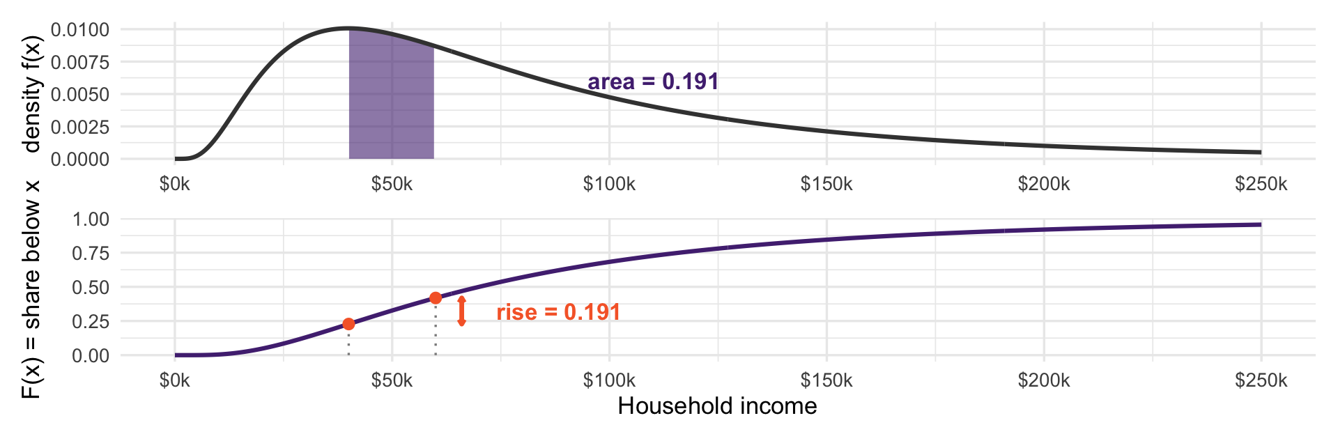
You already use this function: $F(x)$ is the percentile. “The 80th percentile is $131,593” says $F(131{,}593) = 0.8$, and the median is where $F$ crosses 0.5.
An interval probability is the rise in the CDF, which is the same number as the area above it.
The density is the slope of the percentile curve: steep where households pile up, nearly flat out in the tail

Density Is Not Probability

$f_X(x)$ is not $P(X = x)$: we saw that is zero
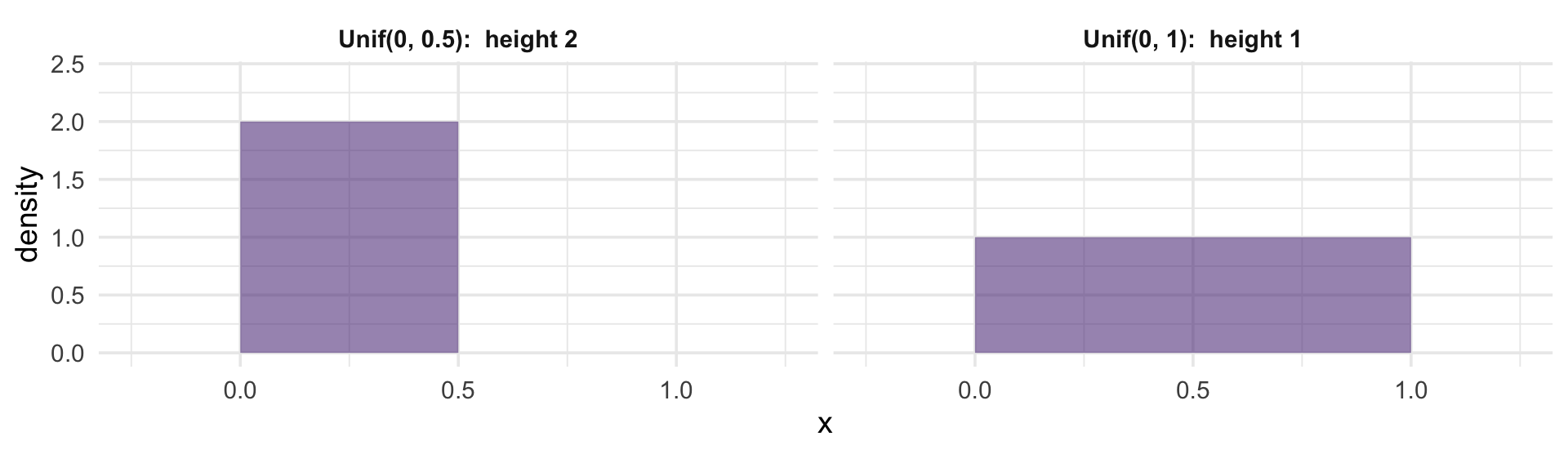
A density can exceed 1. Uniform on $[0, 0.5]$ has density 2 everywhere on its support. Why?
Density is probability per unit of $x$

Think of population density: people per square mile is not a number of people. To get people, you multiply by area. To get probability, you integrate.

Area Is Probability

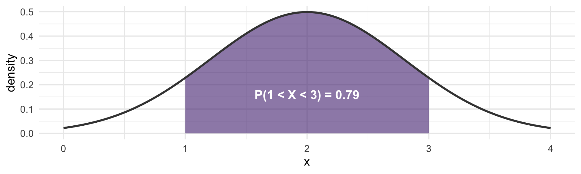
The height at any single point is not a probability.

However, the shaded area is a probability.

Properties of a PDF

Non-negative: $f_X(x) \geq 0$
Integrates to one: $\int_{-\infty}^{\infty} f_X(x)\,dx = 1$

Compare a PMF: non-negative, sums to one. The same rules, with $\int$ for $\sum$.

Note: $P(a < X < b) = P(a \leq X \leq b)$. Why?

Expectation as a Balance Point

Discrete: $\;E[X] = \sum_x x\, p_X(x)$

Continuous: $\;E[X] = \displaystyle\int_{-\infty}^{\infty} x\, f_X(x)\,dx$

Both are “each value, weighted by how likely it is”
Physically: cut the density out of cardboard and $E[X]$ is where it balances on a knife edge
Which is why a long right tail drags the mean: there is weight far out there

Where Does It Balance?

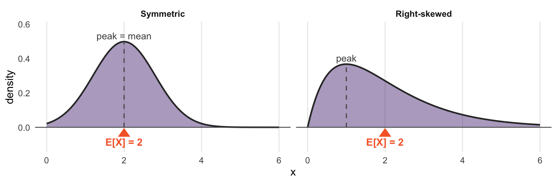
Both of these balance at 2. The symmetric one balances under its peak. The skewed one does not.

The Mean Is Not the Typical Case

On the last slide, the most common value is 1, but the distribution balances at 2
The thin right tail sits far from the fulcrum, so it carries a lot of leverage
Half the probability lies below 1.68 — the median — yet the mean is 2

The mean answers the question “where does the weight balance,” not “what does a typical case look like.”

The Translation Table

Discrete	Continuous
PMF $p_X(x) = P(X = x)$	PDF $f_X(x)$, with $P(X = x) = 0$
$\sum_x$	$\int dx$
$\sum_x p_X(x) = 1$	$\int f_X(x)\,dx = 1$
$E[X] = \sum x\, p_X(x)$	$E[X] = \int x f_X(x)\,dx$
CDF is a step function	CDF is continuous

The concepts are the same, but the mechanics change

The Uniform

The Simplest Continuous Distribution

$X \sim \text{Unif}(a, b)$ — every value in $[a,b]$ is equally likely.

\[f_X(x) = \frac{1}{b-a} \quad \text{for } a \leq x \leq b\]

The density is flat, and its height is whatever makes the area equal 1
$E[X] = \dfrac{a+b}{2}$, the midpoint
$\text{Var}[X] = \dfrac{(b-a)^2}{12}$

Height Is Not Probability

Both have area exactly 1. Narrow the support and the density rises above 1.

Where Uniforms Show Up

Randomization. Assigning treatment by drawing a uniform and splitting at a threshold.
Simulation. Random number generators start from a uniform and make transformations to other distributions
p-values. Under a true null hypothesis, a $p$-value is uniform on $[0,1]$. $p < 0.05$ happens 5% of the time when nothing is going on.

The Normal

The most important distribution (for us)

$X \sim N(\mu, \sigma^2)$, with density

\[f_X(x) = \frac{1}{\sigma\sqrt{2\pi}}\, e^{-\frac{(x-\mu)^2}{2\sigma^2}}\]

You will never integrate this by hand. Nobody can, there is no closed form.
What matters: it is symmetric, unimodal, and described by two numbers
$\mu$ sets the mean, $\sigma^{2}$ sets the variance

The 68–95–99.7 Rule

Worth memorizing.

Standardizing

Any normal becomes the standard normal by subtracting the mean and dividing by the standard deviation:

\[Z = \frac{X - \mu}{\sigma} \sim N(0, 1)\]

$Z$ is a z-score: how many standard deviations from the mean
This is why one table in the back of an old textbook worked for every normal distribution

The Normal in R

dnorm(0)              # density at 0

[1] 0.3989423

pnorm(1.96)           # P(Z <= 1.96)

[1] 0.9750021

qnorm(0.975)          # the value with 97.5% below it

[1] 1.959964

pnorm goes from a value to a probability; qnorm goes back
1.96 is the number behind nearly every 95% confidence interval you have seen
rnorm(n, mean, sd) draws random values

Why Does the Normal Matter So Much?

Very few things in the social world are actually normally distributed
- Income is skewed. Feeling thermometers are bimodal. Counts are not symmetric.
But sample means are approximately normal, almost regardless of what you sampled from
We will see this in more depth when we look at the Central Limit Theorem

For now: the normal matters not because data look normal, but because estimates do. We will return to sampling and the CLT in a few weeks.

A Preview

Same data. The population is nothing like normal. But, the sample means are normal.

You Try

$X \sim \text{Unif}(0, 20)$. What is $E[X]$? What is $P(X > 15)$? What is the height of the density?
Test scores are $N(500, 100^2)$. What share fall between 400 and 600? Use pnorm to check.
What score puts a student at the 90th percentile? Use qnorm.
A polling estimate has standard deviation of 2 points. Roughly how far from the truth would you expect it to be, 95% of the time?

For Next Time

Read: Blitzstein and Hwang, Ch. 5 (remainder)
Next class: joint distributions - describing two random variables at once, and how they move together
- Covariance and correlation
- First big steps towards regression

Discrete	Continuous
PMF \(p_X(x) = P(X = x)\)	PDF \(f_X(x)\), with \(P(X = x) = 0\)
\(\sum_x\)	\(\int dx\)
\(\sum_x p_X(x) = 1\)	\(\int f_X(x)\,dx = 1\)
\(E[X] = \sum x\, p_X(x)\)	\(E[X] = \int x f_X(x)\,dx\)
CDF is a step function	CDF is continuous