POSC 8410: Independence and Dangers of Conditioning

Simpson’s paradox and collider bias

Will Horne

Where We Are

  • Last time: conditioning is the whole point

  • Today: two ways conditioning can go badly wrong

  • Both kept happening all through COVID, which is why today’s reading is Griffith et al. (2020)

Independence

Definition

Events \(A\) and \(B\) are independent if

\[P(A \cap B) = P(A)\,P(B)\]

Equivalently, when \(P(B) > 0\):

\[P(A \mid B) = P(A)\]

In short, Knowing \(B\) tells you nothing about \(A\).

Independent Is Not Disjoint

  • Disjoint: \(A\) and \(B\) cannot both happen. \(P(A \cap B) = 0\).

  • Independent: \(A\) and \(B\) do not inform each other.

These are nearly opposites. If \(A\) and \(B\) are disjoint and both possible, then learning \(B\) happened tells you \(A\) definitely did not - which is the strongest possible dependence.

Very easy to confuse these!

Ten Coin Flips

You flip a fair coin ten times and get ten heads.

What is the probability the eleventh flip is heads?

  • \(0.5\). The coin has no memory.

  • \(P(\text{heads}_{11} \mid \text{ten heads}) = P(\text{heads}_{11})\)

But be careful about which question you are asking. Before any flips, \(P(\text{eleven heads}) = 0.5^{11}\). After ten heads, the remaining uncertainty is one flip.

Independence and Sampling

  • When we draw a random sample, we assume observations are independent and identically distributed (iid)

    • Independent: who I sampled first tells me nothing about who I sample next

    • Identically distributed: every draw comes from the same population

  • This is the assumption that makes much of modern statistics work.

It is also frequently false: clustered samples, snowball samples, repeated measures on the same people, countries in the same region. Violations do not ruin your analysis, but they may change estimation strategy.

Conditional Independence

Definition

\(A\) and \(B\) are conditionally independent given \(C\) if

\[P(A \cap B \mid C) = P(A \mid C)\,P(B \mid C)\]

Once you know \(C\), learning \(B\) tells you nothing further about \(A\).

It Cuts Both Ways

  • Two variables can be dependent overall but independent once you condition

    • Ice cream sales and drowning deaths, given temperature
  • Two variables can be independent overall but dependent once you condition

    • This one is much less intuitive, and we will spend some time on it

Conditioning is not a magic bullet, it can create dependence as easily as it removes it.

Simpson’s Paradox

Two Doctors in Springfield

Dr. Hibbert and Dr. Nick each performed 100 procedures of two kinds. Successes and failures:

Dr. Hibbert Heart Band-Aid
Success 70 10
Failure 20 0
Dr. Nick Heart Band-Aid
Success 2 81
Failure 8 9

Dr. Nick’s overall success rate is 83%. Dr. Hibbert’s is 80%. Which doctor do you want?

The paradox is named for the statistician Edward Simpson, not for the TV show.

Look Within Procedure Type

Heart Band-Aid Overall
Dr. Hibbert 70/90 = 78% 10/10 = 100% 80%
Dr. Nick 2/10 = 20% 81/90 = 90% 83%
  • Dr. Hibbert is better at heart surgery and better at Band-Aid removal

  • Dr. Nick is better overall

  • The catch is the case mix: Hibbert took 90 heart surgeries; Nick took 10. The hard cases went to the better surgeon.

An association can reverse when you condition on a third variable.

Berkeley, 1973

In 1973 the University of California, Berkeley was concerned it faced a lawsuit over gender bias in graduate admissions.

admissions <- as.data.frame(UCBAdmissions) |> as_tibble()

admissions |>
  group_by(Gender) |>
  summarise(applicants = sum(Freq),
            admit_rate = round(100 * sum(Freq[Admit == "Admitted"]) / sum(Freq), 1))
# A tibble: 2 × 3
  Gender applicants admit_rate
  <fct>       <dbl>      <dbl>
1 Male         2691       44.5
2 Female       1835       30.4
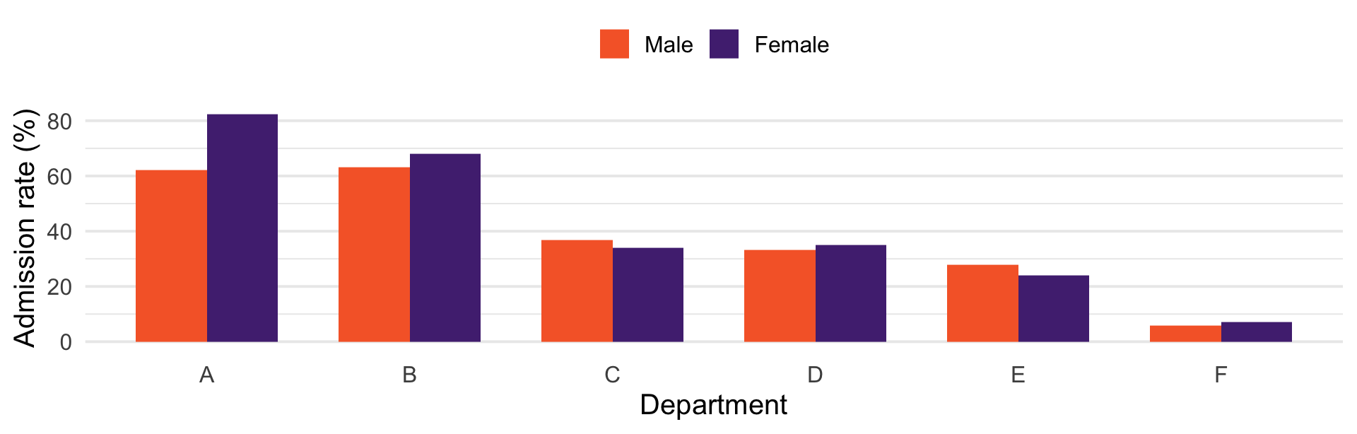
A 14-point gap. That looks bad.

Now Condition on Department

Department Men admitted (%) Women admitted (%)
A 62.1 82.4
B 63.0 68.0
C 36.9 34.1
D 33.1 34.9
E 27.7 23.9
F 5.9 7.0

Women were admitted at a higher rate in four of six departments.

The Picture

So What Happened?

Dept % of applicants who were women Overall admit rate (%)
A 11.6 64.4
B 4.3 63.2
C 64.6 35.1
D 47.3 34.0
E 67.3 25.2
F 47.8 6.4

The Mechanism

  • Women applied disproportionately to the most competitive departments

  • Department is a confounder: it affects both who applies and who is admitted

  • Aggregating over it mixes together departments with wildly different admit rates

Simpson’s paradox: an association that reverses when you condition on a third variable.

Which Number Is Right?

  • That depends entirely on the question

  • “Were women disadvantaged by the admissions committees?” → condition on department. Mostly no.

  • “Were women less likely to get in?” → the aggregate. Yes.

  • “Why did women apply to underfunded, competitive departments?” → a different, and arguably more important, research question

Statistics cannot tell you which question to ask. You have to figure out which question is interesting!

August 2021: “The Vaccines Have Failed”

By mid-August 2021, Israel’s Ministry of Health dashboard showed 515 patients hospitalized with severe COVID - and 58% of them were fully vaccinated.

  • Social media, and some news coverage, drew the obvious conclusion: the vaccines had failed

  • You already know one thing wrong with that: 58% is \(P(\text{vaccinated} \mid \text{severe})\), not \(P(\text{severe} \mid \text{vaccinated})\). With almost 80% of the eligible population vaccinated, the base rate does most of the work (last week!)

  • But there is a second, sneakier problem, even after we condition the right way

Severe Disease, by Vaccination and Age

israel <- tribble(
  ~age,          ~status,        ~severe_per_100k,
  "All (12+)",   "Unvaccinated", 16.4,
  "All (12+)",   "Vaccinated",    5.3,
  "Under 50",    "Unvaccinated",  3.9,
  "Under 50",    "Vaccinated",    0.3,
  "50 and over", "Unvaccinated", 91.9,
  "50 and over", "Vaccinated",   13.6)

israel |>
  pivot_wider(names_from = status, values_from = severe_per_100k) |>
  mutate(efficacy = round(100 * (1 - Vaccinated / Unvaccinated), 1))
# A tibble: 3 × 4
  age         Unvaccinated Vaccinated efficacy
  <chr>              <dbl>      <dbl>    <dbl>
1 All (12+)           16.4        5.3     67.7
2 Under 50             3.9        0.3     92.3
3 50 and over         91.9       13.6     85.2

Israeli MoH dashboard, Aug 15, 2021, ages 12+, severe cases per 100,000; as tabulated by Jeffrey Morris, covid-datascience.com. Rates as published (rounded); from exact counts the efficacies are 67.5 / 91.8 / 85.2

Efficacy is higher in every age group than it is overall.

Age Is the Ommitted Variable

  • Over 90% of Israelis 50+ were vaccinated; 73% of under-50s. 85.7% of the unvaccinated were under 50.

  • So the vaccinated column is full of older, high-risk people, and the unvaccinated column is mostly young, low-risk people. Age drives both vaccination and severe disease

  • Check it with last week’s law of total probability: the unvaccinated overall rate is \(0.857 \times 3.9 + 0.143 \times 91.9 = 16.5 \approx 16.4\). The “All” row is just a weighted average, with very different weights in each column.

For “should I get vaccinated?” the within-age number is the right one - your age is fixed when you decide. Base rates plus weights.

Collider Bias

The Opposite Error

  • Simpson’s paradox: you failed to condition on a confounder, and got a spurious association

  • The obvious lesson would be “condition on everything.”

    • Don’t do this
  • Some variables create bias when you condition on them

These are called colliders - one reason that we don’t just throw a bunch of controls into regression models.

An Admissions Committee

Suppose a program admits students on test scores and essay quality. In the applicant pool the two are unrelated:

set.seed(8410)
applicants <- tibble(test = rnorm(2000), essay = rnorm(2000)) |>
  mutate(admitted = (test + essay) > 1.6)

cor(applicants$test, applicants$essay)
[1] 0.01024972

Essentially zero. Now look only at the students who got in.

Among the Admitted

admitted <- filter(applicants, admitted)

cor(admitted$test, admitted$essay)
[1] -0.6570235

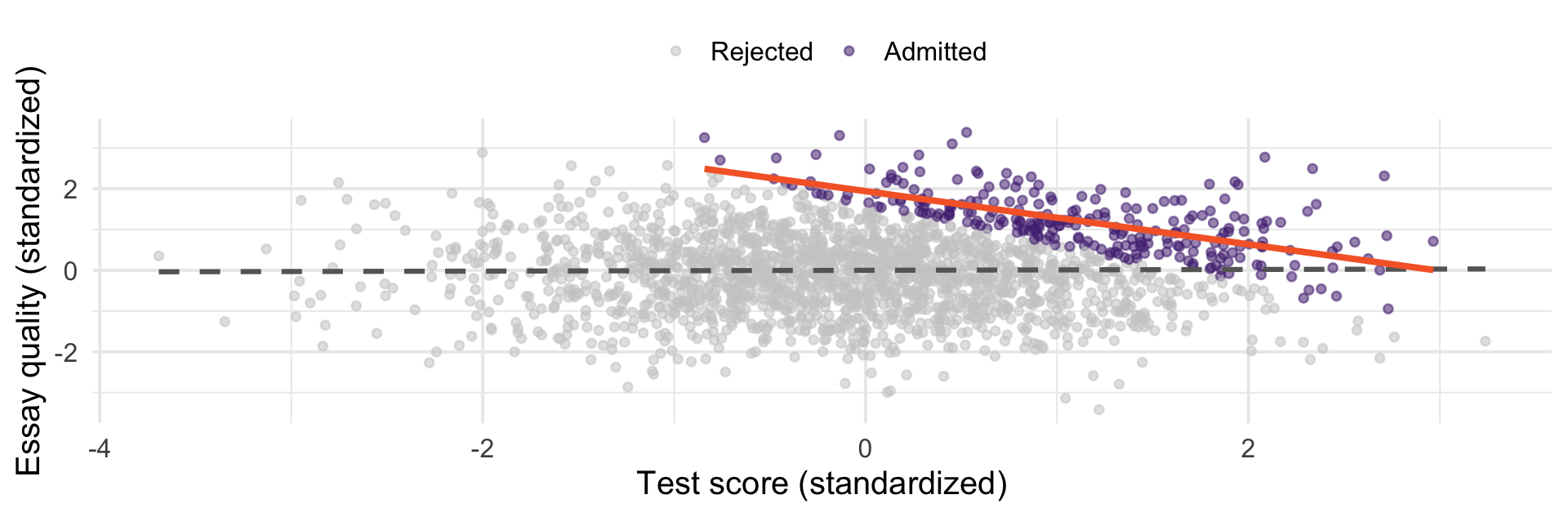
Strongly negative. We invented that correlation by looking only at admitted students.

Seeing It

Dashed line: everyone. Orange line: admitted students only.

Why It Happens

  • To get in with a mediocre test score, your essay had to be excellent

  • To get in with a mediocre essay, your test score had to be excellent

  • Nobody weak on both is accepted

Admission is a collider: both variables point into it. Conditioning on a collider, or on anything downstream of one, induces an association that does not exist in the population.

The Smoker’s Paradox

Spring 2020: studiesfound smokers underrepresented among hospitalized COVID patients. One French hospital study put daily smokers at roughly a quarter of their share of the general population.

  • Researchers proposed nicotine as protective, and patch trials were launched

  • In April 2020, France restricted sales of nicotine patches and gum, capped at a month’s supply, online sales suspended.

  • Today’s reading, Griffith et al. (2020), is about why this whole inference was broken

Where were those studies run? On hospitalized patients.They conditioned on hospitalization.

Build a World Where Smoking Does Nothing

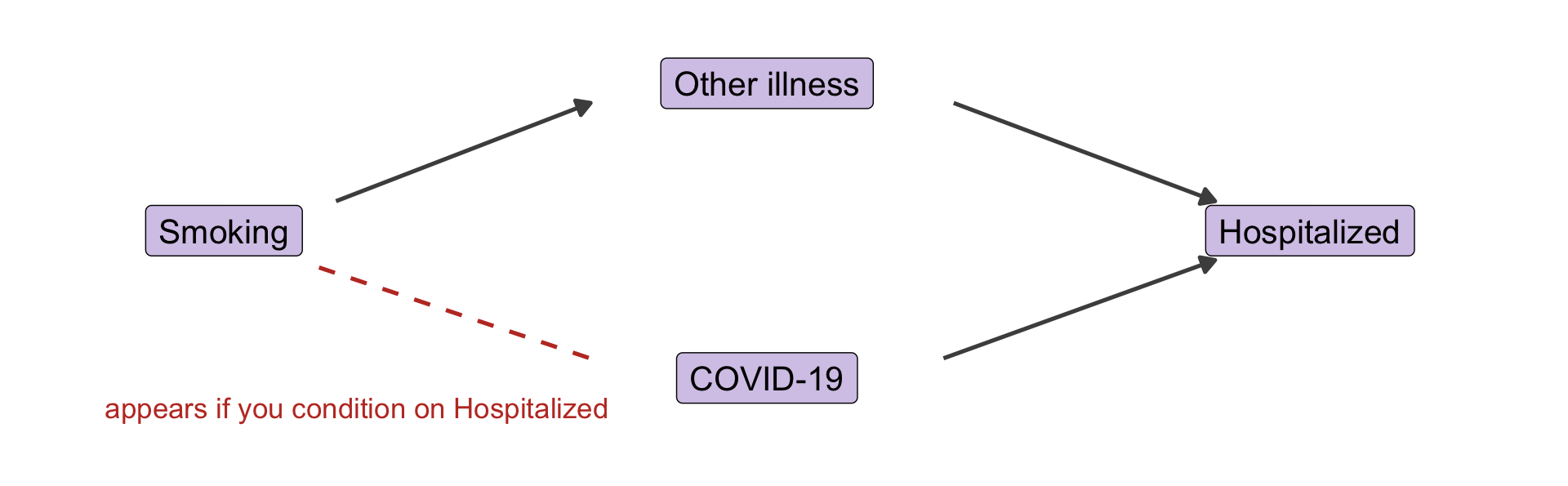
In this simulated world, smoking has no effect on catching COVID. It does cause other illness - and other illness and COVID both send people to the hospital.

set.seed(8410)
n <- 100000
pop <- tibble(
  smoker = rbinom(n, 1, 0.15) == 1,           # 15% of people smoke
  covid  = rbinom(n, 1, 0.10) == 1) |>        # infection independent of smoking
  mutate(
    other_illness = rbinom(n, 1, ifelse(smoker, 0.25, 0.05)) == 1,
    hospitalized  = rbinom(n, 1, 0.02 + 0.30 * covid + 0.25 * other_illness) == 1)

pop |> group_by(smoker) |> summarise(covid_rate = mean(covid))
# A tibble: 2 × 2
  smoker covid_rate
  <lgl>       <dbl>
1 FALSE      0.0981
2 TRUE       0.0976

Now Study Only the Hospital

Do what the spring-2020 studies did: collect your sample from the hospital wards.

hospital <- filter(pop, hospitalized)

hospital |> group_by(smoker) |> summarise(n = n(), covid_rate = mean(covid))
# A tibble: 2 × 3
  smoker     n covid_rate
  <lgl>  <int>      <dbl>
1 FALSE   5238      0.518
2 TRUE    1703      0.326
  • Among hospitalized patients, smokers are about 37% less likely to have COVID - 32.6% vs 51.8%. Nicotine “protects,” in a world we built so that it does nothing.

  • A non-smoker usually needs COVID to end up in the hospital. A smoker has a second path in.

  • Same logic as the admissions committee: two ways into the sample, so among those in, the causes trade off.

The Structure

Hospitalization is a collider: arrows point into it from both sides. Sampling only hospitalized people is conditioning on it, which opens a path between smoking and COVID that does not exist in the population.

Selection Is Conditioning

  • A dean looking only at enrolled students concludes that good test-takers write badly

  • Griffith et al. push the same logic through the whole pandemic: who got tested (health-care workers, constantly), who joins UK Biobank (volunteers, healthier than average), who survives long enough to be studied

  • Any analysis on a selected sample risks this: survey respondents, surviving firms, countries with available data

Selection into your dataset is a form of conditioning, whether or not you chose it.

The Two Errors Together

Confounder Collider
Structure Causes both \(X\) and \(Y\) Caused by both \(X\) and \(Y\)
Do not condition Spurious association Fine
Do condition Fine Spurious association

There is no rule that says “control for more things.” Whether a variable belongs in your model depends on what causes what — which is a theory question, not a data question.

Why We Did This Now

  • In a few weeks you will be running regressions with several predictors

  • Every predictor you add is a decision to condition (or to not condition)

  • Adding a confounder removes bias. Adding a collider creates it. The regression output looks identical either way.

Nothing in the software will warn you. Only your theory of the data generating process can guide you.

For Next Time

  • Read: Probability!, Ch. 2, “Introduction to Random Variables”; Ch. 3 through “Bernoulli”

  • Recommended: Huntington-Klein, The Effect, Ch. 6 (“Causal Diagrams”) — a clear treatment of colliders I know, and it will help enormously in the spring

  • Next class: random variables, and probability distributions